Attention is All You Need

This post offers an interpretation of the paper “Attention is All You Need”. The purpose is to focus on the architecture explained in the article The Annotated Transformer through further reordering and simplification of the PyTorch implementation. The motivation behind this effort is to provide further clarity by starting with the input tensors and working through the model layer by layer rather than starting at a point which is already deep in the weeds (at the encoder). Rather, we will build up to that point by starting at an input sentence, tokenizing and then creating the query, key and value matrices denoted as $Q\:K\:V$. Subsequently, we construct the scaled dot-product attention mechanism before addressing the encoder and decoder. Given this paper serves as a common starting point for those learning about the transformer architecture our objective is to make this post as accessible as possible and easy to understand without large amounts of prior context or knowledge.

Tokenisation, Embedding and Linear Transformation

To get started at the very input of the transformer, let’s consider a simple sentence and an example tokenization for the sentence. While typically we would use a tokenizer for the sake of simplicity as we want to focus on the transformer architecture, we will forgo the implementation. However, a brief explanation of the tokenizer is warranted here: a tokenizer groups relevant neighboring characters together from a given string and converts them into a numerical representation so that they can be used as an input to a neural network. Outlined below is our tensor. We include the batch dimension as to best reflect what happens in a fully developed system:

sentence = ["our", "input", "sentence"]
input_tokens = torch.tensor([[0, 1, 2]]) # Batch, Sequence

Now we can establish the embedding layer of our network. An embedding layer stores a mapping from a vocabulary of tokens to an n-dimensional vector space. In our case we use a vocabulary size of three and an embedding size of three since we are only working with this simple example. However, a typical large language model (LLM) would have a vocabulary size in the tens of thousands and embedding size in the thousands. When passing our tensor to the embedding layer we will get an output of shape: Batch, Sequence, Embedding. Upon examining the tensor after the embedding layer we can see each token in our sequence has been mapped to vector space, with each being represented by an embedding of three values.

vocabulary_size = 3
embedding_size = 3
embedding = torch.nn.Embedding(vocabulary_size, embedding_size)
embedded_sentence = embedding(input_tokens) # Batch, Sequence, Embedding

embedded_sentence
> tensor([[[ 0.6380, -1.4403,  0.9792],   # our
           [-1.5645,  0.0593,  0.4939],   # input
           [-0.1139, -1.0340, -0.0034]]], # sentence
            grad_fn=<EmbeddingBackward0>)

Given our embedded vector, we can now create our $Q\:K\:V$ matrices used in the attention mechanism mentioned in the paper. This is achieved by passing our embedding sentence and feeding it into three seperate fully connected layers to derive the query, key and value matrices.

hidden_size = 64  
linear_transform_Q = torch.nn.Linear(embedding_size, hidden_size)
linear_transform_K = torch.nn.Linear(embedding_size, hidden_size)
linear_transform_V = torch.nn.Linear(embedding_size, hidden_size)

Q = linear_transform_Q(embedded_sentence) # batch, sequence, embedding_size
K = linear_transform_K(embedded_sentence) # """
V = linear_transform_V(embedded_sentence) # """

Scaled Dot-product Attention

Utilizing our $Q\:K\:V$ matrices, we can now address the scaled dot-product attention introduced in the paper. First, the query matrix is mutliplied by the transposed key matrix. Then we divide the resulting matrix by the square root of the transformed embeddings length $\sqrt{d_{k}}$, which is equal to the square-root of the linear transform’s hidden size, in our case 64 -> 8. After this division step the output is optionally masked and put through a softmax function. Then dropout is applied and finally multiplied by the value matrix. The equation shown in the paper is the following, note that we exclude detailing the mask and dropout which we will address later in this article, along with the purpose of the query, key and value matrices and the intuition behind them.

$Attention(Q, K, V) = softmax(\frac{QK^{T}}{\sqrt{d_{k}}})V$

And implemented as Pytorch code

def attention(
      query: torch.Tensor, 
      key: torch.Tensor, 
      value: torch.Tensor, 
      mask: torch.Tensor | None = None, 
      dropout: torch.nn.Module | None = None
    ):
    query_embedding_len = query.size(-1) # same as embedding hidden size (64 in example)
    key = key.transpose(-2, -1) # batch, embedding_size, sequence
    attention_scores = query @ key / math.sqrt(query_embedding_len) # batch, sequence_length, attention_scores

    attention_scores = attention_scores.softmax(dim=-1)

    return attention_scores @ value, attention_scores

Query, Key and Value

Now, we’re familiar with a basic dictionary/hashmap which works by mapping from an exact key to a specific value. Given a specific query we can obtain the associated value.

d = {
   "fun": 10,
   "exciting": 9,
   "boring": -3,
 }
d["fun"] # 10

However, we want to do a lookup based on the meaning of the word and return a vector containing how likely it is that each key in our lookup table is related to our query, or rather how much attention we want to pay to each value based on the query. So for example, let’s take the word “rollercoaster” and assume that we have a 45% match for both “fun” and “exciting” and only a 10% match for “boring”.

query = "rollercoaster"
0.45 * d["fun"] + 0.45 * d["exciting"] + 0.1 * d["boring"] # 5.65

In this example, we have manually created the attention scores based upon how relevant we interpret each key to the query “rollercoaster”. However, how would a model internally arrive at these attention scores? Now if we think back to the previous section we will be reminded that our query and key matrices have the Sequence and Embedding dimensions. The embedding is the significant factor here and having an understanding of how dot products work in relation to the similarity between two vectors helps. However a basic understanding will suffice and the following key ideas are enough to provide intuition into why we use the dot product operation.

• If two vectors are in the same direction their dot product is at it’s largest $n > 0$
• If two vectors are in the opposite direction their dot product is at it’s smallest $n < 0$
• If two vectors are perpendicular their dot product will be zero $n = 0$

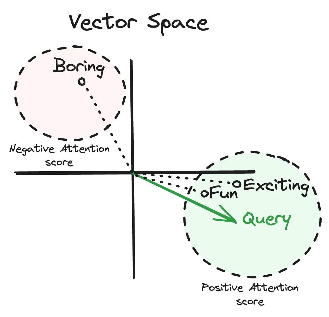
So when we have two word embeddings, our query’s word embedding and our key’s word embedding. When we perform a dot product operation we get a measure of how relevant the key is in relation to the query based on how similar the two are in vector space. To support this we’ve created a desmos visualization with two vectors and their resulting dot product to demonstrate this behaviour. The resulting similarity is called the attention score. What’s happened is that our query embedding is a vector that when mapped into the vector space of the key embedding, is surrounded by tokens that are most relevant to pay attention to. If we change our keys into vectors where our hash-function is now similar to $query \cdot value$ we get an operation which looks like this.

query = [8, -5]
d = {
  [5, -3]: 10, # fun 
  [6, -1]: 9,  # exciting
  [-4, 8]: 3, # boring
}
attention_scores = [8*5 + -5*-3, 8*6 + -5*-1, 8*-4 + -5*8] # [55, 53, -72]

As you can see if our query embedding is close within the key embedding vector space to the “fun” and “exciting” keys it results in a high attention to these values and opposite to the “boring” key resulting in a low attention score. The following diagram shows the above operation’s query and keys in vector space.

Translating our dictionary example in our PyTorch code this is what is happening in the following snippet.

key = key.transpose(-2, -1)
attention_scores = query @ key

Following this, the attention scores are then divided by the square-root of the embedding length and then passed through a softmax function. As the embedding length grows in size, the resultant dot products can become large in magnitude, potentially causing the output values from the softmax to be extremely close to 0 and 1. This in turn may lead to vanishing gradients. This issue is why we scale the attention scores (henced scaled dot product attention). Now, we multiply our attention scores with the values to create a matrix where each element of the sequence contains a new vector embedding that is a weighted combination of the orignal value matrix’s embedding for each word by the attention scores for that particular token.

+ query_embedding_len = query.size(-1)
  key = key.transpose(-2, -1)
- attention_scores = query @ key
+ attention_scores = query @ key / math.sqrt(query_embedding_len)
+ attention_scores = attention_scores.softmax(dim=-1)
+ return attention_scores @ value, attention_scores

We skipped the masking and dropout layer to focus on the explanation of the $Q\:K\:V$ matrices. Dropout is used as expected as a regularization method to prevent the transformer from overfitting. The masking is used in the decoder stack to prevent current predictions from referencing tokens in the future which could result in incorrect sequence generation. We will dive deeper into this when we address the decoder stack.

Multi-Head Attention

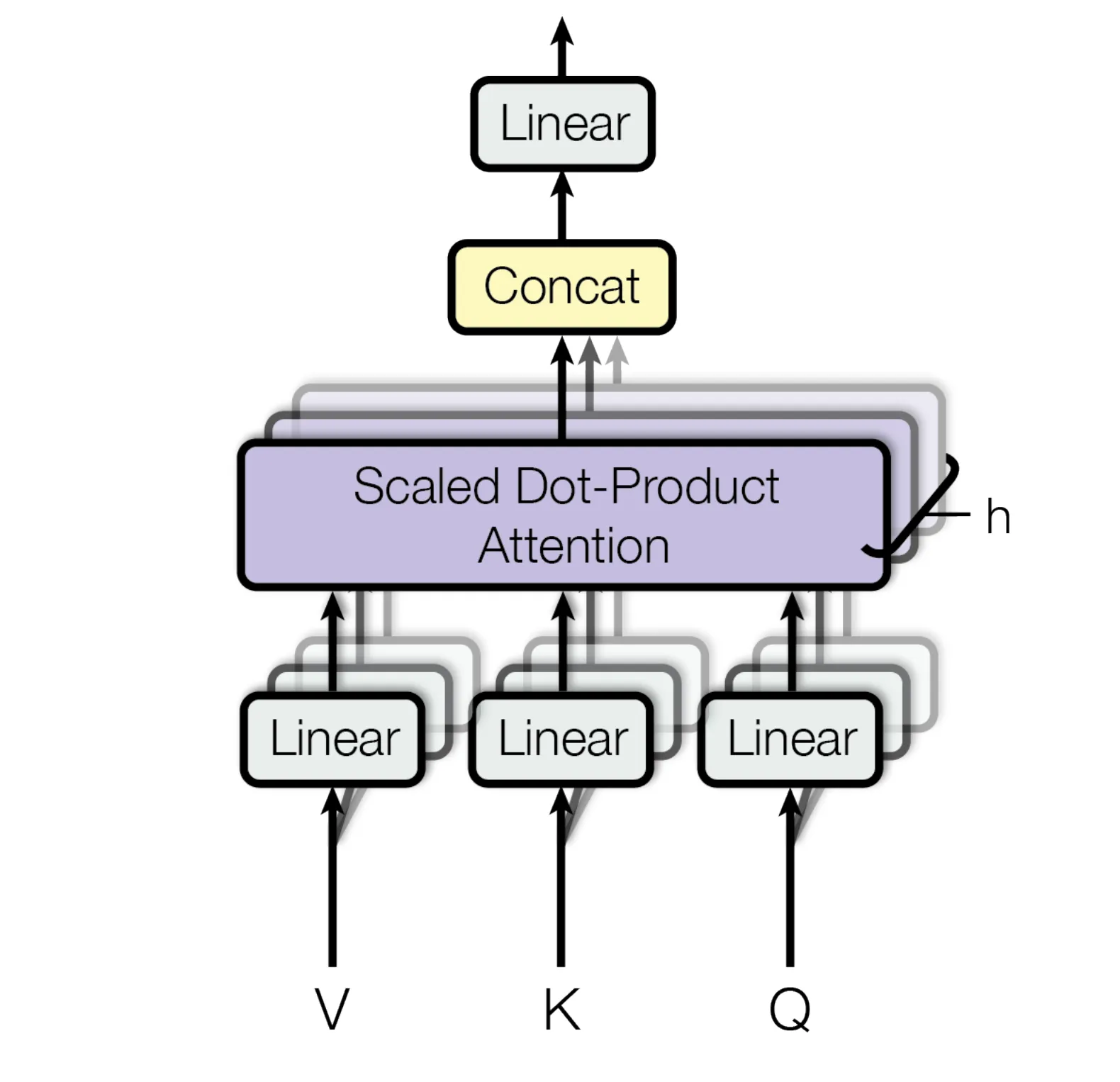
Multi-Head Attention consists of combining our linear transform step and the scaled dot-product attention step into a single function. Together these operations become a single head. Subsequently, applying this function multiple times on the input embedded vector becomes multi-head attention. We take the results from each head and simply concatentate them together, then pass the result through a final linear layer as shown in the following figure. The idea is that the multiple heads create a number of independently modelled word associations with different vector spaces for the $Q\:K\:V$ matrices, this could result in individual heads learning particular relationships such as pronouns to nouns (eg. Her hat) or noun to verb (eg. Door closes). The concatenated results are then put through another linear layer to finalise our multi-head attention

The following python snippet is multihead attention example with 3 heads, and no mask or dropout using the attention function we defined earlier. In this example we use a loop to iterate over each individual head sequentially for simplicity. However, in practice, we would want to parallelise this. Note that we are using the same tensor for the query, key and value, this implementation is correct for the Encoder but will change later in the Decoder. However we will code the head to take in all three matrices such as it will work in both cases.

class Head(torch.nn.Module):
  def __init__(self, input_embedding_size: int, hidden_size: int):
    super().__init__() 
    self.linear_transform_Q = torch.nn.Linear(input_embedding_size, hidden_size)
    self.linear_transform_K = torch.nn.Linear(input_embedding_size, hidden_size)
    self.linear_transform_V = torch.nn.Linear(input_embedding_size, hidden_size)

  def forward(self, Q: torch.Tensor, K: torch.Tensor, V: torch.Tensor) -> torch.Tensor:
    Q = self.linear_transform_Q(x) # batch, sequence, hidden_size
    K = self.linear_transform_K(x) # """
    V = self.linear_transform_V(x) # """
    output, _ = attention(Q, K, V)
    return output

num_heads = 3
input_embedding_size = 3
hidden_size = 64

heads = [Head(input_embedding_size, hidden_size) for _ in range(num_heads)]
fc_out = torch.nn.Linear(hidden_size * num_heads, input_embedding_size * num_heads)

mock_embedded_sentence = torch.randn(1, 3, input_embedding_size * num_heads) # Batch, Sequence, Embedding * Number of Heads
mock_embedded_sentence_split = torch.split(mock_embedded_sentence, num_heads, dim=2)

out = []
for i in range(num_heads):
  input = mock_embedded_sentence_split[i]
  out.append(heads[i](input, input, input))

concat = torch.cat(out, dim=2) # batch, sequence, hidden_size * num_heads
out = fc_out(concat)

Encoder

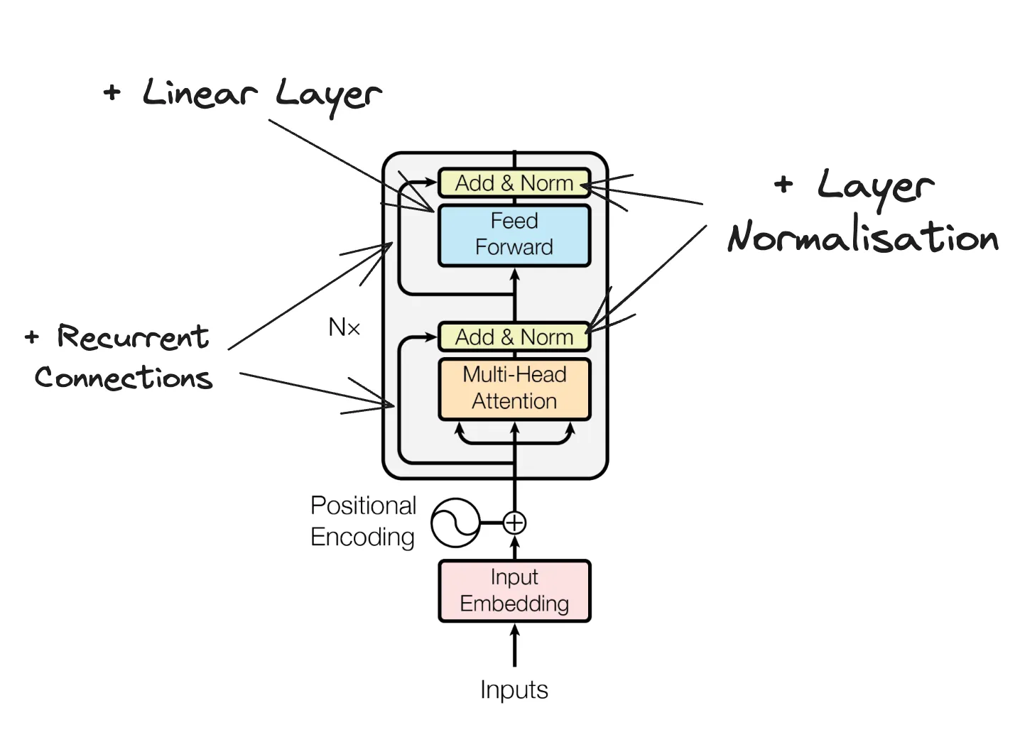
To finish the encoder mechanism we will add the recurrent connections, layer normalization and linear layer as illustrated in the digram from the paper (Note: the positional embedding will be covered independently). We start by making the EncoderTransformerBlock which is contained within the main block of the following diagram and then the Encoder which contains the six repeated transformer blocks.

class EncoderBlock(torch.nn.Module):
  def __init__(self, input_embedding_size: int, num_heads: int, hidden_size: int, forward_expansion: int):
    super().__init__()
    self.num_heads = num_heads

    # Multi-Head Attention
    self.heads = [Head(input_embedding_size, hidden_size) for _ in range(num_heads)]
    self.mha_fc_out = torch.nn.Linear(hidden_size * num_heads, input_embedding_size * num_heads)

    # First Normalisation
    self.norm1 = nn.LayerNorm(input_embedding_size * num_heads)

    # Feed Forward
    self.feed_forward = nn.Sequential(
       nn.Linear(input_embedding_size * num_heads, input_embedding_size * num_heads * forward_expansion),
       nn.ReLU(),
       nn.Linear(input_embedding_size * num_heads * forward_expansion, input_embedding_size * num_heads)
    )

    # Second Normalisation
    self.norm2 = nn.LayerNorm(input_embedding_size * num_heads)

  def forward(self, x):
    # Multi-Head Attention
    split = torch.split(x, self.num_heads, dim=2)
    out = []
    for i in range(self.num_heads):
      input = split[i]
      out.append(heads[i](input, input, input))
    out = torch.cat(out, dim=2) # batch, sequence, hidden_size * num_heads
    out = fc_out(out)

    # First Normalisation
    x = self.norm1(out + x) # Recurrent

    # Feed Forward
    ff = self.feed_forward(x)

    # Second Normalization
    x = self.norm2(ff + x) # Recurrent
    return x

input_embedding_size = 3
num_heads = 3
hidden_size = 64
forward_expansion = 4
sequence_length = 3

encoder = EncoderBlock(
  input_embedding_size, 
  num_heads, 
  hidden_size, 
  forward_expansion
)

input = torch.randn(1, sequence_length, input_embedding_size * num_heads)
output = encoder(input)
output.shape # torch.Size([1, 3, 9]) (same as input size)

We can then easily repeat this block multiple times (in the paper, six) to complete our encoder, eg.

encoder = nn.Sequential(*[
  EncoderBlock(
    input_embedding_size, 
    num_heads, 
    hidden_size, 
    forward_expansion
  ) 
for _ in range(6)])

The Decoder & Masking

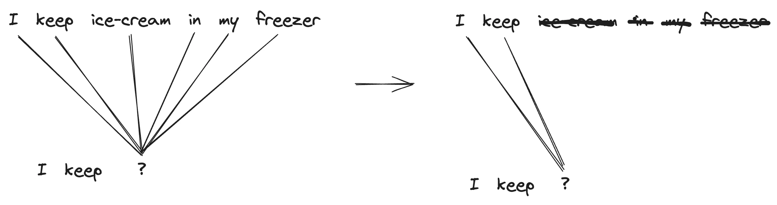
Until now, we have ignored a bit of an issue in our attention mechanism which would be detrimental for model training and inference. Right now our model can see tokens in the future when training. This creates an effect where the models predictions are biased since it can already see output in the future. Take a simple example, ["I", "keep", "ice-cream", "in", "my", "freezer"]. Currently while accessing the value matrix with our attention scores we are allowing the model to include weighting from future tokens in the resulting embedding. This means when training to predict the word “ice-cream” the model is given the additional context “in my freezer” when computing probabilities. However as a generative model at inference time we will not have reliable future tokens predicted yet, this means a models output may utilize its own predicted future values in its internal states to generate subsequent tokens. This can lead to a compounding error effect where inaccuracies in predicting future tokens can propagate and amplify errors in subsequent token predictions.

To solve this, for each prediction we apply a mask so the model can only see the current token, and the tokens leading up to it which in turn reduces the error from incorporating future information prematurely. This makes the model causal which is a common term thrown around in sequence and timeseries problems which in simple terms means that predictions are based solely on preceding information, ensuring that each prediction is influenced only by the data available up to that point in the sequence.

Remember the masking is done on the attention scores so the sentences at the top of the diagram is the model’s internal state not the labels directly. Taking our previous attention function we can now add our mask. We will also add our dropout layer to aid regularization for preventing model overfitting. This completes our scaled dot-product attention function. We update the Head class to utilise these values

def attention(
      query: torch.Tensor, 
      key: torch.Tensor, 
      value: torch.Tensor, 
      mask: torch.Tensor | None = None, 
      dropout: torch.nn.Module | None = None
    ):
    query_embedding_len = query.size(-1) # same as embedding hidden size (64 in example)
    key = key.transpose(-2, -1) # batch, embedding_size, sequence
    attention_scores = query @ key / math.sqrt(query_embedding_len) # batch, sequence_length, attention_scores

+   if mask is not None:
+       scores = scores.masked_fill(mask == 0, -1e9)

    attention_scores = attention_scores.softmax(dim=-1)

+   if dropout is not None:
+       attention_scores = dropout(p_attn)

    return attention_scores @ value, attention_scores


class Head(torch.nn.Module):
  def __init__(self, input_embedding_size: int, hidden_size: int):
    super().__init__() 
    self.linear_transform_Q = torch.nn.Linear(input_embedding_size, hidden_size)
    self.linear_transform_K = torch.nn.Linear(input_embedding_size, hidden_size)
    self.linear_transform_V = torch.nn.Linear(input_embedding_size, hidden_size)

- def forward(self, Q: torch.Tensor, K: torch.Tensor, V: torch.Tensor) -> torch.Tensor:
+ def forward(self, Q: torch.Tensor, K: torch.Tensor, V: torch.Tensor, mask: torch.Tensor | None = None, dropout: torch.nn.Module | None = None) -> torch.Tensor:
    Q = self.linear_transform_Q(x) # batch, sequence, hidden_size
    K = self.linear_transform_K(x) # """
    V = self.linear_transform_V(x) # """
-   output, _ = attention(Q, K, V)
+   output, _ = attention(Q, K, V, mask, dropout)
    return output

and create a new function to generate the mask

def mask(size):
    attn_shape = (1, size, size)
    mask = torch.triu(torch.ones(attn_shape), diagonal=1).type(
        torch.uint8
    )
    return mask == 0

mask(3)
# Output:
# torch.Tensor([[[True, False, False],
#                [True,  True, False],
#                [True,  True,  True]]])

With our attention function now containing masking functionality we can create the decoder block. This block is very similar to the encoder, however we add an additional multi-head attention layer which utilises the masking and in the second attention layer we will use the query matrix from the masked attention layer with the output matrix from the encoder as the key and value. This means we will be using a query which has been masked and will only contain information up to the preceding token thus only allowing information from previous positions in the sequence to influence the generation of each subsequent token, preserving the causal nature of the decoder’s predictions.

class DecoderBlock(nn.Module):
  def __init__(self, input_embedding_size: int, num_heads: int, hidden_size: int, forward_expansion: int):
    super().__init__()
    self.num_heads = num_heads

    # Masked Multi-Head Attention
    self.masked_head = [Head(input_embedding_size, hidden_size) for _ in range(num_heads)]
    self.masked_mha_fc_out = torch.nn.Linear(hidden_size * num_heads, input_embedding_size * num_heads)

    # First Normalisation
    self.norm1 = nn.LayerNorm(input_embedding_size * num_heads)


    # Multi-Head Attention with Encoder's output as Key + Value
    self.unmasked_head = [Head(input_embedding_size, hidden_size) for _ in range(num_heads)]
    self.unmasked_mha_fc_out = torch.nn.Linear(hidden_size * num_heads, input_embedding_size * num_heads)

    # Second Normalisation
    self.norm2 = nn.LayerNorm(input_embedding_size * num_heads)

    # Feed Forward
    self.feed_forward = nn.Sequential(
       nn.Linear(input_embedding_size * num_heads, input_embedding_size * num_heads * forward_expansion),
       nn.ReLU(),
       nn.Linear(input_embedding_size * num_heads * forward_expansion, input_embedding_size * num_heads)
    )

    # Third Normalisation
    self.norm3 = nn.LayerNorm(input_embedding_size * num_heads)

  def forward(self, x, encoder_out, mask):
    # Masked Multi-Head Attention
    split = torch.split(x, self.num_heads, dim=2)
    out = []
    for i in range(self.num_heads):
      input = split[i]
      out.append(self.masked_heads[i](input, input, input))
    out = torch.cat(out, dim=2) # batch, sequence, hidden_size * num_heads
    out = self.masked_mha_fc_out(out)

    # First Normalisation
    x = self.norm1(out + x) # Recurrent


    # Multi-Head Attention with Encoder's output as Key + Value
    split = torch.split(x, self.num_heads, dim=2)
    split_encoder_output = torch.split(encoder_output, self.num_heads, dim=2)
    out = []
    for i in range(self.num_heads):
      input = split[i]
      input_encoder = split_encoder_output[i]
      out.append(self.masked_heads[i](input, input_encoder, input_encoder))
    out = torch.cat(out, dim=2) # batch, sequence, hidden_size * num_heads
    out = self.unmasked_mha_fc_out(out)

    # Second Normalisation
    x = self.norm2(out + x) # Recurrent

    # Feed Forward
    ff = self.feed_forward(x)

    # Third Normalization
    x = self.norm3(ff + x) # Recurrent
    return x

Thus creating our decoder as:

decoder = nn.Sequential(*[
  DecoderBlock(
    input_embedding_size, 
    num_heads, 
    hidden_size, 
    forward_expansion
  ) 
for _ in range(6)])

Positional Encoding

The remaining puzzle piece for our transformer model is the positional encoder. Currently the model has no method of telling which order the tokens appear. This means that for an individual token there is no context present for the model to determine whether the other tokens are within a few words or thousands of words worth of distance. This distance needs to somehow be communicated through to the model. To do this, the paper contains a sinusoidal embedding added to the input embeddings. Adding these sinusoidal embeddings to the word embeddings pushes tokens in close proximity to each other towards a more similar vector space, if we recall back to our dot-product usage in our attention mechanism we will in turn recognise that this will promote higher attention scores between these tokens. The positional encoding used in the paper consists of sin and cosine functions of different frequencies where $i$ is the index of the dimension of the positional encoding

$PE(pos,2i) = sin(\frac{pos}{10000^{2i/dmodel}})$

$PE(pos,2i + 1) = cos(\frac{pos}{10000^{2i/dmodel}})$

And in python, to calculate the positional encoding for a single position

def positional_encoding(position, d_model):
  pos_encoding = np.zeros((1, d_model))
  for i in range(d_model):
    if i % 2 == 0:
      pos_encoding[:, i] = np.sin(position / (10000 ** (i * 2 / d_model)))
    else:
      pos_encoding[:, i] = np.cos(position / (10000 ** ((i-1) * 2 / d_model)))
  return pos_encoding

# The first token in with an embedding size of 8
positional_encoding(0, 8) # [   0,    1,     0,    1, 0, 1, 0, 1]
positional_encoding(1, 8) # [0.84, 0.54, 0.009, 0.99, 0, 1, 0, 1]

# Positions 0, 1 have quite similar vectors

To do this vectorised we compute a constant matrix that we add in the forward step

class PositionalEncoder(nn.Module):
  def __init__(self, d_model, max_len=3): # max len is 3 for example (d_model = embedding_size)
    super().__init__()
    positional_encoding = torch.zeros(max_len, d_model) # sequence_length, encoding_length
    position = torch.arange(0, max_len).unsqueeze(1) # sequence_length
    div_term = torch.exp(
        torch.arange(0, d_model, 2) * -(math.log(10000.0) / d_model)
    ) # encoding_length
    positional_encoding[:, 0::2] = torch.sin(position * div_term) # fill values for even positions
    positional_encoding[:, 1::2] = torch.cos(position * div_term) # fill values for odd positions
    positional_encoding = positional_encoding.unsqueeze(0) # add batch dimension
    self.register_buffer("positional_encoding", positional_encoding)

  def forward(self, x):
    x = x + self.postitional_encoding[:, : x.size(1)].requires_grad_(False)
    return x

positional_encoder = PositionalEncoder(3)

Assembling the Transformer

Now that we have all our necessary components explained and built, we can finally assemble our transformer model. We have our embedding layers for the input and the target sentence. We then add the positional encoding to each of these. We then pass the input sequence to the encoder then pass the target sentence along with the encoder output to the decoder. Finally the output from the decoder is put through a linear layer and a softmax to predict the output at each point in the target sequence. Keep in mind, for simplicity we use a sequence length of three so we do not need to mask the input tensor, however in practice we would have to use a mask to be able to concatenate examples into batches. Without this masking of the inputs the model would pay attention to empty tokens which would negatively affect training.

class Transformer(nn.Module):
  def __init__(self):
    super().__init__()

    # Basic Config
    vocabulary_size = 3
    embedding_size = 3
    num_heads = 6
    hidden_size = 64
    forward_expansion = 4
    sequence_length = 3

    self.input_embedding = torch.nn.Embedding(vocabulary_size, embedding_size)
    self.target_embedding = torch.nn.Embedding(vocabulary_size, embedding_size)

    self.positional_encoder = PositionalEncoder(embedding_size)

    self.encoder = nn.Sequential(*[
      EncoderBlock(
        embedding_size, 
        num_heads, 
        hidden_size, 
        forward_expansion
      ) 
    for _ in range(6)])

    self.decoder = nn.Sequential(*[
      DecoderBlock(
        embedding_size, 
        num_heads, 
        hidden_size, 
        forward_expansion
      ) 
    for _ in range(6)])

    self.linear = nn.Linear(embedding_size
    self.softmax = nn.Softmax()

    self.mask = mask(sequence_length)


  def forward(self, input, target):
    input = self.positional_encoder(self.input_embedding(input))
    target = self.positional_encoder(self.target_embedding(target))

    encoder_output = self.encoder(input) 
    decoder_output = self.decoder(target, encoder_output, self.mask)

    x = self.linear(decoder_output)
    x = self.softmax(x)

    return x

Closing remarks

We hope this blog post has been beneficial in your understanding of the transformer architecture. Please reach out with any issues or feedback.

Thank you, Max van Dijck